Contrastes no paramétricos
Índice
- 1. Contrastes de localización o de homogeneidad
- 2. Contrastes de independencia
- 3. Prueba exacta de Fisher
- 4. Riesgo relativo (RR) y razón de cuotas (odds ratio OR)
\(\newcommand{\mediana}{{\text{Me}}}\) \(\newcommand{\PR}[1]{{\Pr\left[#1\right]}}\) \(\newcommand{\binomial}[2]{{\mathcal B\left(#1,#2\right)}}\) \(\newcommand{\dif}{{\,\mathrm d}}\)
1. Contrastes de localización o de homogeneidad
1.1. Una muestra
- Contrastar la centralización en torno a un valor determinado.
- Comparables al test \(t\)
- Para variables continuas.
- No requieren gausianidad ni tamaño muestral grande.
- Menos potentes que el test \(t\).
1.1.1. Prueba de los signos (o binomial o de la mediana)
- Sea \(X\) una variable aleatoria continua.
- Sea \(\mediana\) la mediana de \(X\). \[ H_0\colon\mediana=M_0\iff F_X(M_0)=\frac12 \qquad H_1\colon\mediana\ne M_0 \]
- La distribución empírica \(F_n(\mediana^-)=\frac{\#\{X_i < \mediana\}}n\) verifica \[F_n(\mediana^-)\xrightarrow{\text{cs}}F_X(\mediana^-)=\frac12\]
- Sea \(U=\#\{X_i < M_0\} = nF_n(M_0^-)\); entonces, \(U\hookrightarrow\mathcal B\left(n,\frac12\right)\).
- Contraste
- Se rechaza \(H_0\) cuando \(F_n(M_0^-)\) es muy diferente de \(\frac12\): \[\text{RC}=\left[F_n(M_0^-)-\frac12 < a_1\right] \cup \left[F_n(M_0^-)-\frac12 > a_2\right]\]
La RC estará formada por valores de \(U\) alejados de \(\frac n2\) \[ \text{RC} = \left[U < c_1 \cup U > c_2\right] \] Por ejemplo, con \(n=14\) y \(\alpha=0.05\):
n = 14
a = 0.05
c1 = qbinom (a/2,   n, 1/2) # c1=3
c2 = qbinom (1-a/2, n, 1/2) # c2=11
tamaño = function (c1, c2)
  pbinom(c1-1,n,1/2) + 1-pbinom(c2,n,1/2)
tamaño(c1,c2)     # 0.01293945
tamaño(c1+1,c2)   # 0.03515625 mejor
tamaño(c1,c2-1)   # 0.03515625 mejor
tamaño(c1+1,c2-1) # 0.05737305 no vale
## => c1=4 c2=11 o bien c1=3 c2=10
binom.test( 2,n) $ p.value # 0'01294
binom.test( 3,n) $ p.value # 0'05737
binom.test( 4,n) $ p.value # 0'1796
binom.test(11,n) $ p.value # 0'05737
binom.test(12,n) $ p.value # 0'01294
- Se puede aplicar a alternativas unilaterales
- \(H_0\colon\mediana \ge M_0\), \(H_1\colon\mediana < M_0\)
- Bajo \(H_0\), \(F_0(M_0)\le F_0(\mediana)=\frac12\)
Se rechaza \(H_0\) si \(F_n(M_0)\) es mucho mayor que \(\frac12\) \[\text{RC}=\left[F_n(M_0)-\frac12 > a_3\right]=\left[U > c_3\right]\]
c3 = qbinom(1-a,n,1/2) # 10
1 - pbinom(c3,n,1/2) # tamaño 0.02868652
## greater == ( F0(M0) > 1/2 )
binom.test (  c3, n, alternative="greater") $ p.value # 0.08978
binom.test (c3+1, n, alternative="greater") $ p.value # 0.02869
\(H_0\colon\mediana \le M_0\), \(H_1\colon\mediana > M_0\) \[\text{RC}=\left[F_n(M_0)-\frac12 < a_4\right]=\left[U < c_4\right]\]
c4 = qbinom(a,n,1/2) # 4
pbinom (  c4, n, 1/2) # 0.08978271
pbinom (c4-1, n, 1/2) # 0.02868652
## less == ( F0(M0) < 1/2 )
binom.test (c4-1, n, alt="less") $ p.value # 0.02869
- \(H_0\colon\mediana \ge M_0\), \(H_1\colon\mediana < M_0\)
- Se puede aplicar a contrastes sobre cualquier cuantil
- Por ejemplo, sea \(H_0\colon Q_1=P_{25}=c_0\), \(H_1\colon P_{25}\ne c_0\)
Sea el estadístico \(U\) = número de observaciones menores que \(c_0\) \[U\stackrel{H_0}\hookrightarrow\mathcal B\left(n,\frac14\right)\]
n = 14 ; a = 0.05
qbinom(c(a/2,1-a/2), n, 1/4) # 1 7
pbinom(0,n,1/4) + 1-pbinom(7,n,1/4) # 0.02812748
binom.test (0, n, 1/4) $ p.value # 0.02812748
binom.test (1, n, 1/4) $ p.value # 0.2126373
binom.test (7, n, 1/4) $ p.value # 0.0560887
binom.test (8, n, 1/4) $ p.value # 0.01030953
Búsqueda automática de la RC
p0 <- 1/4
n  <- 14
ta <- function (c1,c2) pbinom(c1-1,n,p0) + 1-pbinom(c2,n,p0)
al <- 0.05
## explorando sólo los inmediatos
c1 <- qbinom(al/2, n, p0) ; c2 <- qbinom(1-al/2, n, p0)
pr <- c("c1,c2"=ta(c1,c2), "c1+1,c2"=ta(c1+1,c2),
        "c1,c2-1"=ta(c1,c2-1), "c1+1,c2-1"=ta(c1+1,c2-1))
eval(parse(text=paste("c(",names(pmax(pr[pr <= al])),")"))) # 1 7
## búsqueda completa
RC <- names (which (cumsum (sort (setNames (dbinom(0:n,n,p0), 0:n))) <= al))
## "14" "13" "12" "11" "10" "9"  "8"  "0"
- Intervalo de confianza para la mediana (o cualquier cuantil)
- Confianza \(1-\alpha\)
- Se buscan \(r\) y \(s\) tales que \(\Pr[X_{(r)} < \mediana < X_{(s)}] \ge 1-\alpha\)
- \(\Pr[\mediana < X_{(1)}]\) = \(\Pr[\forall i, X_i > \mediana]\) = \(\left(\frac12\right)^n\) = \(\Pr\left[\binomial n{\frac12} = 0\right]\)
- \(\PR{\mediana < X_{(2)}}\) = \(\PR{\mediana < X_{(1)}}\) + \(\PR{X_{(1)}\le\mediana < X_{(2)}}\) = \(\PR{\binomial{n}{\frac12} = 0}\) + \(\PR{\binomial{n}{\frac12} = 1}\) = \(\binom n0\frac1{2^n}\) + \(\binom n1\frac1{2^n}\)
- \(\PR{\mediana < X_{(s)}}\) = \(\sum_{i=0}^{s-1}\PR{\binomial{n}{\frac12}=i}\) = \(\sum_{i=0}^{s-1}\binom ni\frac1{2^n}\)
- \(\PR{X_{(r)} < \mediana < X_{(s)}}\) = \(\PR{\mediana < X_{(s)}}\) \(-\) \(\PR{\mediana < X_{(r)}}\) = \(\sum_{i=r}^{s-1}\binom ni\frac1{2^n}\) \(\ge\) \(1-\alpha\)
El intervalo será \((X_{(r)},X_{(s)})\)
n  <- 14 ; al <- 0.05 ; p0 <- 1/2
pr <- cumsum (sort (setNames (dbinom(0:n,n,p0), 0:n),
                    decreasing = TRUE))
i  <- which (pr >= 1 - al) [1]
ii <- sort (as.numeric (names (pr[1:i])))
r  <- ii[1]              # 3
s  <- ii[length(ii)] + 1 # 11
Si \(p_0=1/2\) la distribución binomial es simétrica, luego hay otra solución posible:
pr <- cumsum (sort (setNames (dbinom(n:0,n,p0), n:0),
                    decreasing = TRUE))
i  <- which (pr >= 1 - al) [1]
ii <- sort (as.numeric (names (pr[1:i])))
r  <- ii[1]              # 4
s  <- ii[length(ii)] + 1 # 12
El cambio de
0:nporn:0se basa en que el algoritmo usado por omisión porsortes estable, luego en caso de empates conserva el orden original.La función
BSDA::SIGN.testde R realiza una interpolación para dar un resultado simétrico, lo que además permite obtener un nivel de significación cercano al deseado aunque, al ser una aproximación, se corre el riesgo de no cumplirlo rigurosamente.
1.1.2. Rangos signados o con signo o de Wilcoxon
- Definiciones
- Rango = posición que ocupa una observación en la muestra ordenada
- Rango de \(X_{(i)}\) es \(i\)
Rangos de \((1.2;7.4;6.2;2.3)\) son \((1;4;3;2)\)
rank (c (1.2, 7.4, 6.2, 2.3)) # 1 4 3 2
- Rango con signo = rango del valor absoluto de la observación,
con el signo original de la observación
- muestra original \((x_1;\dots;x_n)\) = \((-3.5;1.2;0.4;-6.5)\)
- valores absolutos \((|x_1|;\dots;|x_n|)\) = \((3.5;1.2;0.4;6.5)\)
- rangos \((3;2;1;4)\)
rangos signados \((-3;2;1;-4)\)
X <- c (-3.5, 1.2, 0.4, -6.5)
sign (X) * rank (abs (X)) # -3  2  1 -4
- Rango = posición que ocupa una observación en la muestra ordenada
- Contraste sobre la mediana
- Sea \(X\) una variable aleatoria continua y SIMÉTRICA \[ H_0\colon\mediana=\mu=M_0\qquad H_1\colon\mu\ne M_0 \]
- Sea \(D\) = \(X - M_0\) simétrica respecto a cero bajo \(H_0\)
Sean \[ T^+=\sum_{D_i > 0}\text{rango}(|D_i|)\qquad T^-=\sum_{D_i < 0}\text{rango}(|D_i|)\] \[ T^+ + T^- = 1+2+\dots+n=\frac{n(n+1)}2 \] Ejemplo: \(\vec x = (-3.5;1.2;0.4;-6.5)\), \(\mu=0\), rangos con signo \((-3,2,1,-4)\) \[T^+ = 2+1 = 3\qquad T^-=3+4=7\qquad T^++T^-=\frac{4\cdot5}2=10\]
wilcox.test(X,mu=0)$statistic # 3
- Bajo \(H_0\), \(T^+\) verifica
- Toma valores enteros entre \(0\) y \(\frac{n(n+1)}2\)
- Su distribución es simétrica respecto a \(\frac{n(n+1)}4\)
- Su valor tiende a ser cercano al de \(T^-\)
- La región crítica será \[ \text{RC} = \left[T^+ < c_1 \cup T^+ > c_2\right] \]
- Ejemplo de cálculo de probabilidad bajo \(H_0\)
para \(n=4\) y \(\vec r=(3,-1,2,-4)\)
- \(H_0\) \(\implies\) \(f_D(x)=f_D(-x)\) y \(F_D(-x)=1-F_D(x)\)
- \(\PR{\vec R=(3,-1,2,-4)}\) = \(\PR{0 < -D_2 < D_3 < D_1 < -D_4}\) = \(\int_{-\infty}^0 f(d_2) \int_{-d_2}^{\infty} f(d_3) \int_{d_3}^{\infty} f(d_1) \int_{-\infty}^{-d_1} f(d_4) \dif d_4 \dif d_1 \dif d_3 \dif d_2\) = \(\int_{-\infty}^0 f(d_2) \int_{-d_2}^{\infty} f(d_3) \int_{d_3}^{\infty} f(d_1) [1-F(d_1)] \dif d_1 \dif d_3 \dif d_2\) = \(\int_{-\infty}^0 f(d_2) \int_{-d_2}^{\infty} \frac12 f(d_3) [1-F(d_3)]^2 \dif d_3 \dif d_2\) = \(\int_{-\infty}^0 \frac16 f(d_2) [1-F(-d_2)]^3 \dif d_2\) = \(\int_{-\infty}^0 \frac16 f(d_2) F(d_2)^3 \dif d_2\) = \(\frac1{24}[F(0)]^4\) = \(\frac1{24}\left(\frac12\right)^4\)
- Sean \(\pi\) las posibles permutaciones. Entonces
- \(\PR{T^+=0}\) = \(\PR{\pi(-1,-2,-3,-4)}\) = \(4!\frac1{24}\left(\frac12\right)^4\) = \(\left(\frac12\right)^4\)
- \(\PR{T^+=5}\) = \(\PR{\pi(-1,2,3,-4)\cup\pi(1,-2,-3,4)}\) = \(2\cdot4!\frac1{24}\left(\frac12\right)^4\) = \(\left(\frac12\right)^3\)
- Para \(n=4\) \[\PR{T^+=i}= \begin{cases} \left(\frac12\right)^4 & i=0;1;2;8;9;10\\ \left(\frac12\right)^3 & i=3;4;5;6;7 \end{cases} \]
- Las variables \(|D|\) y \(\text{signo}(D)\) son independientes bajo \(H_0\): \( \PR{|D| < x \cap D > 0}\) = \(\PR{0 < D < x}\) = —por la simetría de \(D\)— = \(\frac12\PR{-x < D < x}\) = \(\PR{D > 0}\cdot\PR{|D| < x}\)
- La variable \(T^+\) se expresa como combinación lineal de variables independientes 1: \[ T^+{=}\sum_{r=1}^n rY_{(r)} \qquad Y_i=[D_r > 0]\stackrel{H_0}\hookrightarrow\binomial{1}{\frac12} \]
- \(E(T^+)\) = \(\sum_{r=1}^n r\cdot E(Y_{(r)})\) = \(\sum_{r=1}^n r\cdot \frac12\) = \(\frac{n(n+1)}2\frac12\) =\(\frac{n(n+1)}4\)
- \(\text{Var}(T^+)\) = \(\sum_{r=1}^n r^2\cdot \text{Var}(Y_r)\) = \(\sum_{r=1}^n r^2\cdot \frac14\) = \(\frac{n(n+1)(2n+1)}6\frac14\) =\(\frac{n(n+1)(2n+1)}{24}\)
- Para \(n\gg0\) por la condición de Lindeberg (TCL) \(T^+\) tiene distribución aproximadamente gausiana.
## datos
n <- 15
mu <- 5; sigma <- 1; x <- rnorm (n, mu, sigma)
mu0 <- 4.5
## rangos signados
rs <- rank (abs (x - mu0)) * sign (x - mu0)
Tmas <- sum (rs [rs > 0]) # wilcox.test(x,mu=mu0)$statistic
## Montecarlo
distri <- replicate (1e6, sum ((1:n) * rbinom(n,1,1/2)))
pvalor <- 2 * min (mean (distri <= Tmas), mean (distri >= Tmas))
## por ejemplo: 0.72003
wilcox.test (x, mu=mu0) # p-value = 0.7197
## comprobaciones de gausianidad
shapiro.test (sample (distri, 5000)) # shapiro.test requiere n<5001
qqnorm (distri) # con n=15 se curvan las colas; PP plot:
mu.t <- n*(n+1)/4
dt.t <- sqrt(n*(n+1)*(2*n+1)/24)
plot (ppoints (length(distri)), pnorm(sort(distri),mu.t,dt.t))
abline (0, 1, col=2) # se aprecia el escalonamiento central; densidad:
hist (distri, prob=TRUE)
plot (function(x)dnorm(x,mu.t,dt.t), 0, n*(n+1)/2, col=2, add=TRUE)
1.2. Dos muestras independientes
- \(X\hookrightarrow F_X\), \(Y\hookrightarrow F_Y\)
- \(H_0\colon F_X=F_Y\), \(H_1\colon F_X\ne F_Y\)
1.2.1. \(\chi^2\) de homogeneidad
- para variables discretas finitas con valores \(C_1,\dots,C_k\)
- muestras aleatorias simples \(\vec X\) = \((X_1,\dots,X_{n_X})\); \(\vec Y\) = \((Y_1,\dots,Y_{n_Y})\)
- tamaño muestral conjunto \(n\) = \(n_X\) + \(n_Y\)
- sean \(p_{Xj}=\PR{X=C_j}\), \(p_{Yj}=\PR{Y=C_j}\)
- \(H_0\colon \forall\,j,\, p_{Xj}=p_{Yj}=p_{j}\), \(H_1\colon \exists\,j,\,p_{Xj}\ne p_{Yj}\)
tabla de frecuencias observadas \(O_{ij}=n_{ij}\), \(i\in\{X,Y\}\), \(j\in\{1,\dots,k\}\)
\(C_1\) \(C_2\) \(\dots\) \(C_k\) totales \(X\) \(n_{X1}\) \(n_{X2}\) \(\dots\) \(n_{Xk}\) \(n_X\) \(Y\) \(n_{Y1}\) \(n_{Y2}\) \(\dots\) \(n_{Yk}\) \(n_Y\) totales \(n_1\) \(n_2\) \(\dots\) \(n_k\) \(n\) - verosimilitud bajo \(H_1\) \[ \mathcal L(\vec n, \vec p_X, \vec p_Y) \propto \prod_{i\in\{X,Y\}}\prod_{j=1}^{k}p_{ij}^{n_{ij}} \] estimaciones máximo-verosímiles \[ \hat p_{ij} = \frac{n_{ij}}{n_i} \]
- verosimilitud bajo \(H_0\) \[ \mathcal L(\vec n, \vec p) \propto \prod_{j=1}^{k}p_{j}^{n_{j}} \] estimaciones máximo-verosímiles \[ \hat p_{j} = \frac{n_j}{n} \]
- frecuencias absolutas esperadas \[ E_{ij} = n_i\hat p_j = \frac{n_in_j}n \]
- razón de verosimilitudes \( \Lambda(\vec n) \) = \( \dfrac {\mathcal L(\vec n, \hat{\vec p})} {\mathcal L(\vec n, \hat{\vec p}_X, \hat{\vec p}_Y)}\) = \( \displaystyle\prod_{i\in\{X,Y\}}\prod_{j=1}^k \left(\dfrac{n_j/n}{n_{ij}/n_i}\right)^{n_{ij}} \) = \( \displaystyle\prod_{i\in\{X,Y\}}\prod_{j=1}^k \left(\dfrac{n_i n_j/n}{n_{ij}}\right)^{n_{ij}} \) = \( \displaystyle\prod_{i\in\{X,Y\}}\prod_{j=1}^k \left(\dfrac{E_{ij}}{O_{ij}}\right)^{O_{ij}} \)
- \(G\) = \(-2\ln\Lambda\) = \(\displaystyle\sum_{i\in\{X,Y\}}\sum_{j=1}^k O_{ij}\ln\frac{O_{ij}}{E_{ij}}\)
- RC = \([G > c]\)
- \(G\) \(\stackrel{H_0}{\hookrightarrow}\) \(\chi^2_{2(k-1)-(k-1)}\) = \(\chi^2_{k-1}\)
- \(D\) = \(\displaystyle\sum_{i\in\{X,Y\}}\sum_{j=1}^k \frac{(O_{ij}-E_{ij})^2}{E_{ij}}\)
- RC = \([D > c]\)
- \(D\) \(\stackrel{H_0}{\hookrightarrow}\) \(\chi^2_{k-1}\)
1.2.2. KS
- \(H_0\colon F_X=F_Y=F_0\), \(H_1\colon F_X\ne F_Y\)
- muestras aleatorias simples \(\vec X=(X_1,\dots,X_{n_X})\), \(\vec Y=(Y_1,\dots,Y_{n_Y})\)
- \(D_{n_X n_Y}\) = \(\displaystyle \sup_{x\in\mathbb R} |F_{n_X}(x)-F_{n_Y}(x)|\) = \(\displaystyle \sup_{x\in\mathbb R} \left|\frac{\#\{X_i\le x\}}{n_X}-\frac{\#\{Y_i\le x\}}{n_Y}\right|\) = \(\displaystyle \sup_{x\in\mathbb R} \left|\frac{\#\{F_0(X_i)\le F_0(x)\}}{n_X}-\frac{\#\{F_0(Y_i)\le F_0(x)\}}{n_Y}\right|\) = \(\displaystyle \sup_{0 < u < 1} \left|\frac{\#\{U_i\le u\}}{n_X}-\frac{\#\{U_i\le u\}}{n_Y}\right|\)
- de libre distribución bajo \(H_0\) pues \[F_0(X)\;\stackrel{H_0}{\equiv}\;F_0(Y)\;\stackrel{H_0}{\equiv}\;\mathcal U(0;1)\]
- para variables continuas; puede haber problemas si hay empates
ejemplo
X <- c (2, 1, 2.5, 4)
Y <- c (3, 3.1, 2.3, 3.7, 4.5)
XY <- c (X, Y) # muestra conjunta
## XY ordenada: 1 2 2.3 2.5 3 3.1 3.7 4 4.5
## FnX = (1, 2, 2, 3, 3, 3, 3, 4, 4) / 4
## FnY = (0, 0, 1, 1, 2, 3, 4, 4, 5) / 5
D <- max (abs (ecdf(X)(XY) - ecdf(Y)(XY))) # 3/4 - 1/5 = 0,55
1 - psmirnov (D, c(length(X),length(Y)))   # 0.4285714
ks.test (X, Y)
##      Two-sample Kolmogorov-Smirnov test
##
## data:  X and Y
## D = 0.55, p-value = 0.4286
## alternative hypothesis: two-sided
1.2.3. Prueba de la mediana
- Distribución hipergeométrica
- Sea una población con \(n_1\) individuos de tipo 1 y \(n_2\) de tipo 2.
- Sea una muestra sin reposición de tamaño \(n\).
- Sea \(U\) el número de individuos de tipo 1 en la muestra.
- \(U\) sigue una distribución hipergeométrica, \(U\hookrightarrow\mathcal H(n_1,n_2,n)\).
\(U\) toma valores entre \(\max\{0,n-n_2\}\) y \(\min\{n,n_1\}\); por ejemplo
- \(\mathcal H(4;6;5)\) toma valores \(\{0;1;2;3;4\}\)
- \(\mathcal H(6;4;5)\) toma valores \(\{1;2;3;4;5\}\)
\[\PR{U=u} = \frac{\binom{n_1}{u}\binom{n_2}{n-u}}{\binom{n_1+n_2}{n}}\] \[E(U) = n\frac{n_1}{n_1+n_2}\] \[\text{Var}(U) = n\frac{n_1}{n_1+n_2}\frac{n_2}{n_1+n_2}\frac{n_1+n_2-n}{n_1+n_2-1}\]
- Contraste de la mediana
- Dos variables continuas \(X\) y \(Y\).
- Sendas muestras aleatorias simples \(\vec X=(X_1,\dots,X_{n_X})\) y \(\vec Y=(Y_1,\dots,Y_{n_Y})\).
- Hipótesis \(H_0\colon\mediana_X=\mediana_Y\), \(H_1\colon\mediana_X\ne\mediana_Y\),
- Sea \(M\) la mediana de la muestra conjunta \((\vec X, \vec Y)\)
- Sea \(U\) el número de \(X_i\) menores que \(M\); \(i=1,\dots,n_X\)
- Sea \(t-U\) el número de \(Y_j\) menores que \(M\), \(j=1,\dots,n_Y\); luego \(t=\#\{X_i < M\} + \#\{Y_j < M\}\)
- RC = \([U < c_1] \cup [U > c_2]\)
- Se extraen \(t\) individuos, sin reposición, de \(n_X\) de \(X\) y \(n_Y\) de \(Y\). \[ U \hookrightarrow \mathcal H(n_X,n_Y,t) \] luego \(U\) es de distribución libre.
Ejemplo:
nX <- 10
nY <- 9
n <- nX + nY
t <- 9
## 0 <= u <= 9
## bajo H0 la distribución de U es
round (setNames (dhyper (0:t, nX, nY, t), 0:t), 5)
##       0       1       2       3       4       5       6       7       8       9
## 0.00001 0.00097 0.01754 0.10912 0.28643 0.34372 0.19095 0.04676 0.00438 0.00011
## > sum(dhyper(7:9,nX,nY,t))
## [1] 0.05125679
## > sum(dhyper(c(0:2,8:9),nX,nY,t))
## [1] 0.02301414
## alfa=0,05 => RC = {0;1;2;8;9}
- Contraste de localización
- \(Y\,\stackrel{\mathcal L}{\equiv}\,X+\theta\) \(\iff\) \(F_Y=F_{X+\theta}\) \(\iff\) \(F_X=F_{Y-\theta}\)
- \(H_0\colon \theta=\theta_0\) \(H_1\colon \theta\ne\theta_0\)
- \(H_0\) \(\iff\) \(F_X=F_{Y-\theta_0}\) \(\implies\) \(\mediana(X) = \mediana(Y-\theta_0)\)
- ejemplo
- \(\vec x=(2;1;2.5;4)\), \(\vec y=(3;3.1;2.3;3.7;4.5)\)
- muestra conjunta \((\vec x; \vec y-2)\) = \((2;1;2.5;4;1;1.1;0.3;1.7;2.5)\)
- mediana conjunta = \(1.7\)
\(t\) = —número de menores que \(1.7\)— = 4
> dhyper (0:4, 4, 5, 4)
[1] 0.039682540 0.317460317 0.476190476 0.158730159 0.007936508
- RC = \([U \in \{0;4\}]\); \(\PR{\text{RC}}\) = \(0.0476\) \(\le\) \(0.05\)
- \(U\) = —número de \(x_i\) menores que \(1.7\)— \(\implies\) \(u=1\) \(\notin\) RC \(\implies\) no se rechaza \(H_0\)
1.2.4. Prueba de Mann y Whitney
- Muy usado.
- \(H_0\colon X\,\stackrel{\mathcal L}{\equiv}\,Y\), \(H_1\colon X\,\stackrel{\mathcal L}{\not\equiv}\,Y\)
- Muestras \(\vec x=(x_1,\dots,x_{n_X})\) y \(\vec y=(y_1,\dots,y_{n_Y})\)
- \(Z_{ij}\) = \([X_i < Y_j]\) \(\hookrightarrow\) \(\mathcal B\left(1,\PR{X < Y}\right)\)
- \(Z_{ij}\) \(\stackrel{H_0}\hookrightarrow\) \(\mathcal B\left(1,\frac12\right)\) pues \(\PR{X < Y\mid H_0}\) = \(\int_{\mathbb R} \int_{x}^{\infty}f(x)f(y)\dif y \dif x\) = \(\int_{\mathbb R} f(x)\int_{x}^{\infty}f(y)\dif y \dif x\) = \(\int_{\mathbb R} f(x)[1-F(x)]\dif x\) = \(\left[-\frac12[1-F(x)]^2\right]_{x=-\infty}^{x=\infty}\) = \(\frac12\)
- \(U\) = \(\sum_{i=1}^{n_X}\sum_{j=1}^{n_Y}Z_{ij}\) \(\in\) \(\{0,\dots,n_Xn_Y\}\)
- \(H_0\) \(\implies\) \(\PR{X < Y}=\frac12\) \(\implies\) \(E(U)=\sum_{i=1}^{n_X}\sum_{j=1}^{n_Y}E(Z_{ij})\) = \(\frac{n_X n_Y}2\) \(\implies\) \(U\approx \frac{n_X n_Y}{2}\) \(\implies\) RC = \([U < c_1] \cup [U > c_2]\)
- ejemplo
- \(\vec x\) = \((2;1;2.5)\), \(\vec y\) = \((2.4;3.1;2.3;3.7)\)
- \(n_X = 3\), \(n_Y = 4\)
- muestra conjunta ordenada: \((1x;2x;2.3y;2.4y;2.5x;3.1y;3.7y)\) \(\implies\) \((x,x,y,y,x,y,y)\)
- \(u\) = 2 + 2 + 3 + 3 = 4 + 4 + 2 = 10
- bajo \(H_0\)
- el número de posibles ordenaciones de tres \(x\) y cuatro \(y\) es \(\binom{7}{3}\) = \(\frac{7!}{3!4!}\) = 35
- todas las ordenaciones son igualmente probables: \(\PR{xxxyyyy}\) = \(\dots\) = \(\PR{yyyyxxx}\)
- \(0\le u\le12\)
- \(u=0\) \(\iff\) \((yyyyxxx)\)
- \(u=1\) \(\iff\) \((yyyxyxx)\)
- \(u=2\) \(\iff\) \((yyxyyxx)\) \(\cup\) \((yyyxxyx)\)
- \(u=3\) \(\iff\) \((yxyyyxx)\) \(\cup\) \((yyxyxyx)\) \(\cup\) \((yyyxxxy)\)
- …
la distribución de \(U\) es simétrica respecto a \(6\)
- \(U(xyxxyyy)\) = 10 \(\iff\) \(U(yyyxxyx)\) = \(2\) = \(12-10\)
> dwilcox (0:12, 3, 4)
 [1] 0.02857143 0.02857143 0.05714286 0.08571429 0.11428571 0.11428571
 [7] 0.14285714 0.11428571 0.11428571 0.08571429 0.05714286 0.02857143
[13] 0.02857143
> dwilcox (0:12, 3, 4) * 35
 [1] 1 1 2 3 4 4 5 4 4 3 2 1 1
- bajo \(H_0\)
- \(Z_{ij}\) depende de \(Z_{ik}\): \(E(Z_{ij}Z_{ik})\) = \(\PR{Z_{ij}=1\cap Z_{ik}=1}\) = \(\PR{X_i < \min\{Y_j,Y_k\}}\) = \(\displaystyle\int_{-\infty}^{\infty} f(x)\int_x^{\infty}2f(y)[1-F(y)]\dif y\dif x\) = \(\displaystyle\int_{-\infty}^{\infty}f(x) \left[-[1-F(y)]^2\right]_{y=x}^{y=\infty}\dif x\) = \(\displaystyle\int_{-\infty}^{\infty}f(x)[1-F(x)]^2\dif x\) = \(\left[-\frac13[1-F(x)]^3\right]_{x=-\infty}^{x=\infty}\) = \(\frac13\) \(\neq\) \(\frac12\cdot\frac12\) = \(E(Z_{ij})\cdot E(Z_{ik})\)
- \(Z_{ij}\) depende de \(Z_{lj}\): \(E(Z_{ij}Z_{lj})\) = \(\PR{\max\{X_i,X_l\} < Y_j}\) = \(\frac13\)
- \(Z_{ij}\) no depende de \(Z_{lk}\): \(E(Z_{ij}Z_{lk})\) = \(\PR{X_i < Y_j\cap X_l < Y_k}\) = \(\PR{X_i < Y_j}\cdot\PR{X_l < Y_k}\) = \(E(Z_{ij})\cdot E(Z_{lk})\) = \(\frac14\)
- \(\text{Var}(U)\) = \(E(U^2)-E^2(U)\) = \(\displaystyle E\left[\left(\sum_{i=1}^{n_X} \sum_{j=1}^{n_Y}Z_{ij}\right)^2\right]-E^2(U)\) = \(\displaystyle E\left[\left(\sum_{i=1}^{n_X} \sum_{j=1}^{n_Y}Z_{ij}\right) \cdot \left(\sum_{l=1}^{n_X} \sum_{k=1}^{n_Y}Z_{lk}\right)\right]-E^2(U)\) = \(\displaystyle E\left[\left(\sum_{i=1}^{n_X} \sum_{j=1}^{n_Y}Z_{ij}\right) \cdot \left( Z_{ij}+\sum_{k\ne j}Z_{ik}+\sum_{l\ne i}Z_{lj} +\sum_{l\ne i}\sum_{k\ne j}Z_{lk} \right)\right]-E^2(U)\)= \(\displaystyle \sum_{i=1}^{n_X} \sum_{j=1}^{n_Y}E\left[Z_{ij}^2\right]\)+ \(\displaystyle\sum_{i=1}^{n_X} \sum_{j=1}^{n_Y}\sum_{k\ne j}E[Z_{ij}Z_{ik}]\)+ \(\displaystyle\sum_{i=1}^{n_X} \sum_{j=1}^{n_Y}\sum_{l\ne i}E[Z_{ij}Z_{lj}]\)+ \(\displaystyle\sum_{i=1}^{n_X} \sum_{j=1}^{n_Y}\sum_{l\ne i}\sum_{k\ne j} E[Z_{ij}Z_{lk}]\) \(-\) \(E^2(U)\)= \(n_X n_Y\frac12\) + \(n_X n_Y (n_Y-1)\frac13\)+ \(n_X n_Y (n_X-1)\frac13\) + \(n_X n_Y (n_X-1) (n_Y-1)\frac14\) \(-\) \(\left(\frac{n_X n_Y}2\right)^2\)= \(\frac{n_X n_Y (n+1)}{12}\)
Maxima 5.44.0 http://maxima.sourceforge.net
using Lisp GNU Common Lisp (GCL) GCL 2.6.12
Distributed under the GNU Public License. See the file COPYING.
Dedicated to the memory of William Schelter.
The function bug_report() provides bug reporting information.
(%i1) EZij : 1/2 $

(%i2) EZij2 : EZij $

(%i3) EU : nX*nY*EZij $

(%i4) EZijZik : 1/3 $

(%i5) EZijZlj : 1/3 $

(%i6) EZijZlk : 1/4 $

(%i7) VarU : nX*nY*EZij2 + nX*nY*(nY-1)*EZijZik +
  nX*nY*(nX-1)*EZijZlj + nX*nY*(nX-1)*(nY-1)*EZijZlk - EU^2 $

(%i8) factor(VarU) ;
                              nX nY (nY + nX + 1)
(%o8)                         -------------------
                                      12
\(U\) es asintóticamente gausiana
x <- rnorm (50)
y <- rnorm (50, 0.6)
wilcox.test (x, y)
wilcox.test (x, y, exact=TRUE)
	Wilcoxon rank sum test with continuity correction

data:  x and y
W = 672, p-value = 6.857e-05
alternative hypothesis: true location shift is not equal to 0


	Wilcoxon rank sum exact test

data:  x and y
W = 672, p-value = 4.782e-05
alternative hypothesis: true location shift is not equal to 0
(De
?wilcox.test) By default (if ‘exact’ is not specified), an exact p-value is computed if the samples contain less than 50 finite values and there are no ties. Otherwise, a normal approximation is used.
1.2.5. Prueba de Wilcoxon
- Asignar rangos a la muestra conjunta y sumarlos: \(R_X\) = \(\displaystyle \sum_{i=1}^{n_X}\text{rango}(X_i)\) ; \(R_Y\) = \(\displaystyle \sum_{i=1}^{n_Y}\text{rango}(Y_i)\) ; \(R_X\) + \(R_Y\) = \(\frac{n (n+1)}2\)
- Si \(\forall\,i,j\), \(x_i < y_j\), entonces \(R_X\) = \(r_{\min}\) = \(1\) + \(\dots\) + \(n_X\) = \(\frac{n_X(n_X+1)}2\)
- Si \(\forall\,i,j\), \(x_i > y_j\), entonces \(R_X\) = \(r_{\max}\) = \((n_Y+1)\) + \(\dots\) + \((n_Y+n_X)\) = \(n_X n_Y+\frac{n_X(n_X+1)}2\) = \(n_X \left(n_Y+\frac{n_X+1}2\right)\)
- Es una trasformación biyectiva de la \(U\) de Mann y Whitney: \(R_Y\) = \(R_{Y_{(1)}}\) + \(R_{Y_{(2)}}\) + \(\dots\) + \(R_{Y_{(n_Y)}}\) = \(U_1+1\) + \(U_2+2\) + \(\dots\) + \(U_{n_Y}+n_Y\) = \(U\) + \(1\) + \(2\) + \(\dots\) + \(n_Y\) = \(U\) + \(\displaystyle\frac{n_Y(n_Y+1)}2\) donde \(R_{Y_{(j)}}\) es el rango de la \(j\)-ésima observación de \(\vec Y\) ordenada y \(U_j\) = \(\#\{X_i < Y_{(j)}\}\)
- \(H_0\colon X\,\stackrel{\mathcal L}{\equiv}\,Y\), \(H_1\colon X\,\stackrel{\mathcal L}{\not\equiv}\,Y\) \(\implies\) RC = \([R_X < c_1]\cup[R_X > c_2]\)
> X <- c(2,1,2.5,4) ; Y <- c(3,3.1,2.3,3.7,4.5)
> nX <- length(X) ; nY <- length(Y)
> names(X) <- rep("X",nX) ; names(Y) <- rep("Y",nY)
> (XY <- names (sort (c (X, Y))))
[1] "X" "X" "Y" "X" "Y" "Y" "Y" "X" "Y"
> (Rx <- sum (which (XY == "X")))
[1] 15
> (Ry <- sum (which (XY == "Y")))
[1] 30
> (U <- sum (sapply (X, function(Xi) sapply (Y, function(Yj) Xi < Yj))))
[1] 15
> ## otra forma de calcular U
> sum(sapply(setdiff(which(XY=="Y"),1),function(j)sum(XY[1:(j-1)]=="X")))
[1] 15
> Ry - nY*(nY+1)/2
[1] 15
> (Umin <- nX*(nX+1)/2)
[1] 10
> (W <- U - Umin)
[1] 5
> wilcox.test (X, Y)

        Wilcoxon rank sum exact test

data:  X and Y
W = 5, p-value = 0.2857
alternative hypothesis: true location shift is not equal to 0
1.3. Dos muestras relacionadas / pareadas
1.3.1. Continuas
tanto la prueba de los signos como la la prueba de Wilcoxon de una muestra pueden aplicarse a la diferencia de dos muestras pareadas, considerando \(M=0\)
> ?sleep
> X <- sleep$extra[sleep$group==1]
> Y <- sleep$extra[sleep$group==2]
> length(X) ; length(Y)
[1] 10
[1] 10
> shapiro.test(X-Y)$p.value
[1] 0.03334161
> sum(X<Y) ; sum(X<=Y) # por redondeo, hay un empate
[1] 9
[1] 10
> binom.test(10,10)$p.value
[1] 0.001953125
> binom.test(9,10)$p.value
[1] 0.02148438
- \(H_0\)
- (necesaria)
- \(X-Y\) es simétrica respecto al \(0\)
- (suficiente)
\((X,Y)\) es intercambiable (lo que implica \(F_X=F_Y\))
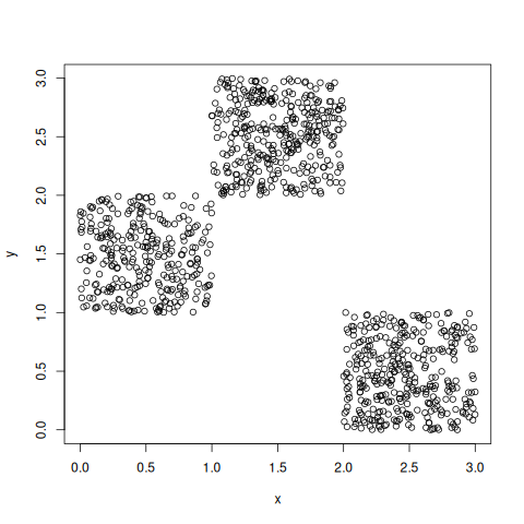
ejemplo de distribución conjunta con \(F_X=F_Y\) pero sin intercambiabilidad:
n <- 1000
x <- runif(n,0,3)
y <- runif(n,0,1) - (x<1) + 2*(x<2)
plot (x, y)
ejemplo de distribución de P-valores bajo \(F_X=F_Y\) pero sin intercambiabilidad:
> n <- 30
> dist <- t(replicate(1e6,
+ {
+     x <- runif(n,0,3)
+     y <- runif(n,0,1) - (x<1) + 2*(x<2)
+     c (b = binom.test (sum(x<y), n) $ p.value,
+        w = wilcox.test (x, y, paired=TRUE) $ p.value)
+ }))
> summary(dist)
        b                 w
 Min.   :0.00000   Min.   :0.0000
 1st Qu.:0.01612   1st Qu.:0.2129
 Median :0.09874   Median :0.4522
 Mean   :0.21396   Mean   :0.4727
 3rd Qu.:0.36159   3rd Qu.:0.7151
 Max.   :1.00000   Max.   :1.0000
> colMeans(dist<0.05)
       b        w
0.432120 0.071572
- Wilcoxon
en R son equivalentes
wilcox.test (x, y, paired=TRUE)
wilcox.test (x-y, mu=0)
1.3.2. Binarias - Prueba de McNemar
- Experimento Bernoulli en dos situaciones diferentes para datos pareados.
- Equivale a
- Q de Cochran con \(k=2\)
- prueba de los signos con \(2\) muestras
Ejemplo: proporción de individuos que presenta una característica \(A\), antes y después de cierto tratamiento.
antes \ después \(A\) \(\bar A\) sumas \(A\) \(a\) \(b\) \(n_{A\cdot}\) \(\bar A\) \(c\) \(d\) \(n_{\bar A\cdot}\) sumas \(n_{\cdot A}\) \(n_{\cdot\bar A}\) \(n\) - \(H_0\) : \(\Pr[A\mid\text{antes}]\) = \(\Pr[A\mid\text{después}]\)
- \(H_1\) : \(\Pr[A\mid\text{antes}]\) \(\ne\) \(\Pr[A\mid\text{después}]\)
- Estimaciones: \(\widehat\Pr[A\mid\text{antes}]\) = \(\dfrac{a+b}n\), \(\widehat\Pr[A\mid\text{después}]\) = \(\dfrac{a+c}n\)
- \(H_0\) \(\implies\) \(b\approx c\)
- promedio \(m\) = \(\dfrac{b+c}2\)
- estadístico \(M\) = \(\dfrac{(b-m)^2+(c-m)^2}m\) = \(\dfrac{2(b-m)^2}m\) = \(\dfrac{\left(b-\dfrac{b+c}2\right)^2}{\dfrac{b+c}4}\) = \(\dfrac{(b-c)^2}{b+c}\)
- RC = \([M > c]\)
- Si se supone conocido \(b+c\) (el número de individuos que cambian) entonces \(b\) \(\stackrel{H_0}{\hookrightarrow}\) \(\mathcal B(b+c,1/2)\) \(\xrightarrow[b+c\to\infty]{\mathcal L}\) \(\mathcal N\left(\dfrac{b+c}2;\sqrt{\dfrac{b+c}4}\right)\) \(\implies\) \(\dfrac{b-\dfrac{b+c}2}{\sqrt{\dfrac{b+c}4}}\) \(\stackrel{\sim}{\hookrightarrow}\) \(\mathcal N(0;1)\) \(\implies\) \(\dfrac{\left(b-\dfrac{b+c}2\right)^2}{\dfrac{b+c}4}\) = \(M\) \(\stackrel{\sim}{\hookrightarrow}\) \(\chi^2_1\)
Ejemplo médico
- respuesta: sufrir o no hipoglucemias
- cada individuo:
- una noche con control normal
- otra noche con control automático
normal \ autom. no hipo. hipoglucemia no hipo. 20 7 hipoglucemia 22 5 - \(H_0\) : \(\Pr[\text{hipo}\mid\text{normal}]\) = \(\Pr[\text{hipo}\mid\text{auto}]\) ; \(H_1\) : \(\Pr[\text{hipo}\mid\text{normal}]\) \(\ne\) \(\Pr[\text{hipo}\mid\text{auto}]\)
- \(M\) = \(\dfrac{(22-7)^2}{22+7}\) \(\approx\) \(7.76\)
1 - pchisq (7.76, 1) # aproximación asintótica
mcnemar.test (matrix(c(20,22,7,5),2), correct=FALSE) # ídem
mcnemar.test (matrix(c(20,22,7,5),2)) # corrección por continuidad
2 * pbinom (7, 22+7, 1/2) # P-valor exacto
## lo mismo que correct=FALSE
friedman.test(do.call(rbind,rep(list(c(0,0),c(0,1),c(1,0),c(1,1)),c(20,22,7,5))))
[1] 0.005341596

	McNemar's Chi-squared test

data:  matrix(c(20, 22, 7, 5), 2)
McNemar's chi-squared = 7.7586, df = 1, p-value = 0.005346


	McNemar's Chi-squared test with continuity correction

data:  matrix(c(20, 22, 7, 5), 2)
McNemar's chi-squared = 6.7586, df = 1, p-value = 0.00933

[1] 0.008130059

	Friedman rank sum test

data:  do.call(rbind, rep(list(c(0, 0), c(0, 1), c(1, 0), c(1, 1)), c(20, 22, 7, 5)))
Friedman chi-squared = 7.7586, df = 1, p-value = 0.005346
1.4. \(k\) muestras independientes
- poblaciones \(X_1\hookrightarrow F_1\), …, \(X_k\hookrightarrow F_k\) independientes
- \(H_0:F_1=\dots=F_k\), \(H_1:\exists\,i,j,\,F_i\ne F_j\)
- muestras \(\vec x_1\), …, \(\vec x_k\); \(\vec x_i\) = \((x_{i1},\dots,x_{in_i})\)
- \(n\) = \(n_1 + \dots + n_k\)
1.4.1. Prueba \(\chi^2\) de homogeneidad
- \(X\) variable discreta finita (o agrupada)
- \(X\) toma valores \(C_1\), …, \(C_r\)
- \(p_{ij}\) = \(\Pr[X_i = C_j]\)
- \(H_0:\forall\,j\in\{1,\dots,r\}\), \(p_{1j}=\dots=p_{kj}\)
tabla de frecuencias observadas \(O_{ij}\) = \(n_{ij}\)
\(C_1\) \(\dots\) \(C_r\) totales \(X_1\) \(n_{11}\) \(\dots\) \(n_{1r}\) \(n_{1\cdot}\) \(\vdots\) \(\vdots\) \(\vdots\) \(\vdots\) \(\vdots\) \(X_k\) \(n_{k1}\) \(\dots\) \(n_{kr}\) \(n_{k\cdot}\) totales \(n_{\cdot1}\) \(\dots\) \(n_{\cdot r}\) \(n\) - verosimilitud bajo \(H_1\) \[\mathcal L(\vec n,\vec p_1,\dots,\vec p_k) \propto \prod_{i=1}^k\prod_{j=1}^r p_{ij}^{n_{ij}}\] EMV \(\hat p_{ij}\) = \(\frac{n_{ij}}{n_{i\cdot}}\)
- verosimilitud bajo \(H_0\) \[\mathcal L(\vec n,\vec p) \propto \prod_{j=1}^r p_{ij}^{n_{\cdot j}}\] EMV \(\hat p_{j}\) = \(\frac{n_{\cdot j}}{n}\)
- frecuencia esperada bajo \(H_0\): \(E_{ij}\) = \(n_i\hat p_j\) = \(\frac{n_{i\cdot}n_{\cdot j}}n\)
- razón de verosimilitudes \(\Lambda(\vec n)\) = \(\displaystyle \frac{\mathcal L(\vec n,\hat{\vec p})} {\mathcal L(\vec n,\hat{\vec p}_1,\dots,\hat{\vec p}_k)}\) = \(\displaystyle \prod_i\prod_j \left(\frac{n_{\cdot j}/n}{n_{ij}/n_{i\cdot}}\right)^{n_{ij}}\) = \(\displaystyle \prod_i\prod_j \left(\frac{n_{i\cdot}n_{\cdot j}/n}{n_{ij}}\right)^{n_{ij}}\) = \(\displaystyle \prod_i\prod_j \left(\frac{E_{ij}}{O_{ij}}\right)^{O_{ij}}\)
- \(G\) = \(-2\ln\Lambda\) = \(2\sum_i\sum_j O_{ij}\ln{\frac{O_{ij}}{E_{ij}}}\)
- RC = \([G > c]\)
- \(G\) \(\xrightarrow[\mathcal L]{H_0}\) \(\chi^2_{k(r-1)-(r-1)}\) = \(\chi^2_{(k-1)(r-1)}\) asintóticamente; la aproximación es buena si \(E_{ij}\ge5\) \(\forall\,i,j\).
- \(D\) = \(\sum_i\sum_j\frac{(O_{ij}-E_{ij})^2}{E_{ij}}\)
- RC = \([D > c]\)
- \(D\) \(\xrightarrow[\mathcal L]{H_0}\) \(\chi^2_{(k-1)(r-1)}\) asintóticamente; la aproximación es buena si \(E_{ij}\ge5\) \(\forall\,i,j\).
1.4.2. Prueba de la mediana
- \(H_0:\mediana_1=\dots=\mediana_k\), \(H_1:\exists\,i,j,\;\mediana_i\ne\mediana_j\)
- Sea \(M\) la mediana de la muestra conjunta.
- Sea \(U_i\) = \(\#\{X_{ij} < M\}\)
- Sea \(t\) = \(\sum_i U_i\) = \(\lfloor \frac n 2\rfloor\)
Tabla de frecuencias
\(X_1\) \(\dots\) \(X_k\) totales \(\#\{x_{ij} < M\}\) \(u_1\) \(\dots\) \(u_k\) \(t\) \(\#\{x_{ij}\ge M\}\) \(n_1-u_1\) \(\dots\) \(n_k-u_k\) \(n-t\) totales \(n_1\) \(\dots\) \(n_k\) \(n\) - Se aplica un \(\chi^2\) de Pearson
- Denótese \(O_{i1}=u_i\) y \(O_{i2}=n_i-u_i\)
- \(E_{i1}\) = \(n_i\widehat\Pr_0[X_i < M]\) = \(n_i\frac tn\), \(E_{i2}\) = \(n_i\widehat\Pr_0[X_i\ge M]\) = \(n_i\frac {n-t}n\)
- \(O_{i2}-E_{i2}\) = \(n_i-u_i-n_i\frac{n-t}n\) = \(-u_i+n_i\frac tn\) = \(-(O_{i1}-E_{i1})\)
- \(D\) = \(\sum_{i=1}^k\sum_{j=1}^2\frac{(O_{ij}-E_{ij})^2}{E_{ij}}\)
= \(\sum_i\left(U_i-n_i\frac tn\right)^2
\left(\frac1{E_{i1}}+\frac1{E_{i2}}\right)\)
= \(\sum_i\left(U_i-n_i\frac tn\right)^2
\left(\frac1{n_i\frac tn}+\frac1{n_i\frac{n-t}n}\right)\)
= \(n^2\sum_i\frac{\left(U_i-\frac{n_it}n\right)}{n_i t(n-t)}\)
- RC = \([D > c]\)
- \(D\) \(\xrightarrow[\mathcal L]{H_0}\) \(\chi^2_{k-1}\)
1.4.3. Prueba de Kruskal y Wallis
- Muy usado.
- \(H_0:F_1=\dots=F_k\), \(H_1:\exists\,i,j,\,F_i\ne F_j\)
- Sea \(R_{ij}\) el rango de \(x_{ij}\) en la muestra conjunta.
- \(R_i\) = \(\sum_{j=1}^{n_i}R_{ij}\) suma de rangos para \(i\)
- \(\bar R_i\) = \(\frac{R_i}{n_i}\) rango medio para \(i\)
- \(\bar R\) = \(\frac1n\sum_i n_i\bar R_i\) = \(\frac{n+1}2\) rango medio global
- Bajo \(H_0\)
- Los rangos son invariantes con la trasformación \(U_i\) = \(F_0(X_i)\) \(\hookrightarrow\) \(\mathcal U(0,1)\)
- Se debe cumplir que \(\bar R_i\) \(\approx\) \(\bar R\) = \(\frac{n+1}2\) \(\forall\,i\)
- Análisis de varianza sobre los rangos
- SCT = \(\sum_i\sum_j(R_{ij}-\bar R)^2\) = \(\sum_i\sum_j\left((R_{ij}-\bar R_i) + (\bar R_i-\bar R)\right)^2\) = \(\sum_i\sum_j\left(R_{ij}-\bar R_i\right)^2\) + \(\sum_i\sum_j\left(\bar R_i-\bar R\right)^2\) = \(\sum_i\sum_j\left(R_{ij}-\bar R_i\right)^2\) + \(\sum_i n_i\left(\bar R_i-\bar R\right)^2\) = SCE + SCF
- SCT es constante; depende sólo de \(n\): SCT = \(\sum_{i=1}^n\left(i-\frac{n+1}2\right)^2\) = \(\sum_{i=1}^n i^2 - n\left(\frac{n+1}2\right)^2\) = \(n\frac{n^2-1}{12}\)
- Estadístico del contraste
\(H\) = \(\displaystyle\frac{12}{n(n+1)}\sum_{i=1}^kn_i\left(\bar R_i-\frac{n+1}2\right)^2\)
= \(\displaystyle \frac{\text{SCF}}{\frac{\text{SCT}}{n-1}}\)
- RC = \([H > c]\)
- \(H\) es de libre distribución bajo \(H_0\)
- Generaliza la prueba de Wilcoxon
- Considerando dos muestras (la \(i\) frente al resto): \(R_i\) \(\xrightarrow[\mathcal L]{H_0}\) \(\mathcal N\left(\frac{n_i(n+1)}2,\sqrt{\frac{n_i(n-n_i)(n+1)}{12}}\right)\) \(\implies\) \(\frac{\left(\bar R_i-\frac{n+1}2\right)^2}{\frac{(n-n_i)(n+1)}{12n_i}}\) = \(\frac{n_i\left(\bar R_i-\frac{n+1}2\right)^2}{\frac{(n-n_i)(n+1)}{12}}\) \(\xrightarrow[\mathcal L]{H_0}\) \(\chi_1^2\)
Las \(\bar R_i\) son dependientes pues \(\sum_i n_i \bar R_i\) = \(\frac{n(n+1)}2\) luego se pierde un grado de libertad: \(H\) = \(\displaystyle \frac{12}{n(n+1)} \sum_{i=1}^k n_i \left(\bar R_i-\frac{n+1}2\right)^2\) \(\xrightarrow[\mathcal L]{H_0}\) \(\chi^2_{k-1}\)
## comprobación de la distro asintótica mediante montecarlo
m <- 100; k <- 4; g <- rep(1:k,each=m)
n <- m*k; n. <- rep(m,k) # == table(g)
H <- function (x, g)
{
    rangos <- rank(x)
    rango. <- tapply(rangos, g, mean)
    12/n/(n+1)*sum(n.*(rango.-(n+1)/2)^2)
}
distri <- replicate (1e5,
{
    x <- runif(n)
    H(x,g)
})
rbind (quantile(distri, pr <- c(1,5,10,50,90,95,99)/100),
       qchisq(pr, k-1))
            1%        5%       10%      50%      90%      95%      99%
[1,] 0.1175384 0.3547309 0.5895572 2.372027 6.243953 7.801314 11.26462
[2,] 0.1148318 0.3518463 0.5843744 2.365974 6.251389 7.814728 11.34487
Ejemplo
- \(\vec x_1\) = \((2;1;2.5;4)\) \(\implies\) \(n_1=4\)
- \(\vec x_2\) = \((3;3.1;2.3;3.7;4.5)\) \(\implies\) \(n_2=5\)
- \(\vec x_3\) = \((2.1;1.3;2.4;4.1)\) \(\implies\) \(n_3=4\)
x1 = c (2, 1, 2.5, 4)
x2 = c (3, 3.1, 2.3, 3.7, 4.5)
x3 = c (2.1, 1.3, 2.4, 4.1)
conjunta = stack (list (a=x1, b=x2, c=x3))
n.i = table (conjunta$ind)
k = length (n.i)
n = nrow (conjunta)
r = rank (conjunta$values)
r.medios = tapply (r, conjunta$ind, mean)
(H = 12 / (n*(n+1)) * sum (n.i * (r.medios - (n+1)/2) ^ 2))
1 - pchisq (H, k-1) # p-pvalor
kruskal.test (values ~ ind, conjunta)
[1] 2.175824
[1] 0.3369192

	Kruskal-Wallis rank sum test

data:  values by ind
Kruskal-Wallis chi-squared = 2.1758, df = 2, p-value = 0.3369
- Empates
- Pueden aparecer por redondeos.
- A \(t\) observaciones empatadas, con rangos \(i\), \(i+1\), …, \(i+t-1\) se les asigna su rango medio \(\dfrac{i+(i+1)+\dots+(i+t-1)}t\) = \(\dfrac{i\cdot t+(1+2+\dots+t-1)}t\) = \(\dfrac{i\cdot t+\dfrac{(t-1)t}2}t\) = \(\dfrac{2i+t-1}2\)
- El rango medio global \(\bar R\) no cambia.
La corrección por los \(t\) empates en la SCT vale \(\displaystyle\sum_{j=0}^{t-1}(i+j)^2-\sum_{j=0}^{t-1}\left({2i+t-1\over2}\right)^2\) = \(\displaystyle\sum_{j=0}^{t-1}(i+j)^2-t\left({2i+t-1\over2}\right)^2\) = \(\dfrac{t(t^2-1)}{12}\) = \(\dfrac{t^3-t}{12}\)
(%i7) factor (nusum ((i+j)^2, j, 0, t-1) - t * ((2*i+t-1)/2)^2) ;
                               (t - 1) t (t + 1)
(%o7)                          -----------------
                                      12
- Si hay \(g\) grupos de empates, con \(t_j\) observaciones empatadas cada uno, la SCT corregida vale SCT\(^*\) = SCT \(-\) \(\displaystyle\frac1{12}\sum_{j=1}^gt_j^3-t_j\)
- Los \(t_1,\dots,t_g\) pueden obtenerse en R mediante
table - Cuando los empates se producen dentro de la misma población \(i\in\{1,\dots,k\}\), el estadístico \(H\) no se modifica.
- Estadístico corregido \(H^*\) = \((n-1)\dfrac{\text{SCF}}{\text{SCT}^*}\) = \(\dfrac{H}{1-\dfrac{\sum_{j=1}^g(t_j^3-t_j)}{n^3-n}}\)
Contrastes a posteriori: prueba de Dunn
- \(H_0:F_1=\dots=F_k\), \(\iff\) \(\displaystyle\bigcap_{i,j}H_0^{ij}:F_i=F_j\)
\[\bar R_i\xrightarrow[\mathcal L]{H_0} \mathcal N\left(\frac{n+1}2,\sqrt{\frac{(n-n_i)(n+1)}{12n_i}}\right)\]
- RC para \(H_0^{ij}:F_i=F_j\) \[\displaystyle \left[\frac {\bar R_i-\bar R_j} {\sqrt{\frac{n(n+1)}{12}\left(\frac1{n_i}+\frac1{n_j}\right)}} > z_{1-\alpha^*}\right]\] con \(\alpha^*=\dfrac\alpha{\binom k 2}\)
dunn.test::dunn.test (list (x1, x2, x3))
FSA::dunnTest (values ~ ind, conjunta)
Error in loadNamespace(x) : there is no package called ‘dunn.test’
Error in loadNamespace(x) : there is no package called ‘FSA’
Contrastes a posteriori: Wilcoxon por parejas
pairwise.wilcox.test (conjunta$values, conjunta$ind)
	Pairwise comparisons using Wilcoxon rank sum exact test

data:  conjunta$values and conjunta$ind

  a    b
b 0.86 -
c 0.89 0.86

P value adjustment method: holm
1.5. \(k\) muestras relacionadas
1.5.1. Prueba de Friedman
- Sea \(\vec X\) = \((X_1,\dots,X_k)\) un vector aleatorio.
- \(H_0:F_1=\dots=F_k\), \(H_1:\exists\,i,j,\,F_i\ne F_j\)
Muestra \(\vec X_1,\dots,\vec X_n\) aleatoria simple de \(\vec X\) con \(\vec X_i\) = \((X_{i1},\dots,X_{ik})\)
individuo \(X_1\) \(\dots\) \(X_k\) \(1\) \(x_{11}\) \(\dots\) \(x_{1k}\) \(\vdots\) \(\vdots\) \(\vdots\) \(\vdots\) \(n\) \(x_{n1}\) \(\dots\) \(x_{nk}\) Rangos intraindividuo
individuo \(X_1\) \(\dots\) \(X_k\) sumas \(1\) \(R_{11}\) \(\dots\) \(R_{1k}\) \(R_{1\cdot}\) \(\vdots\) \(\vdots\) \(\vdots\) \(\vdots\) \(\vdots\) \(n\) \(R_{n1}\) \(\dots\) \(R_{nk}\) \(R_{n\cdot}\) sumas \(R_{\cdot 1}\) \(\dots\) \(R_{\cdot k}\) \(R_{\cdot\cdot}\) - \(R_{\cdot\cdot}\) = \(\dfrac{nk(k+1)}2\)
- \(\text{SCT}=\sum_{i=1}^n\sum_{j=1}^k\left(R_{ij}-\frac{k+1}2\right)^2 =\frac{n\,(k-1)\,k\,(k+1)}{12}\)
- Estadístico del contraste basado en la dispersión de \(R_{\cdot j}\): \(F\) = \(\displaystyle \frac{12}{nk(k+1)} \sum_{j=1}^k\left(R_{\cdot j}-\frac{n(k+1)}2\right)^2\) = \(\displaystyle \frac {\sum_{j=1}^k\left(R_{\cdot j}-\frac{n(k+1)}2\right)^2} {\frac{\text{SCT}}{k-1}}\)
- RC = \([F > c]\)
- Bajo \(H_0\)
- \(R_{\cdot j}\) deberían ser similares
\(F\) es de libre distribución, \(F\) \(\xrightarrow[\mathcal L]{H_0}\) \(\chi^2_{k-1}\)
## comprobación de la distribución asintótica
k <- 3 # número de variables
cova <- matrix(c(1.000, 0.872, 0.818,
                 0.872, 1.000, 0.963,
                 0.818, 0.963, 1.000),
               3)
mu <- c(1.0, 1.1, 1.1) # medias teóricas
n  <- 100 # tamaño muestral
X  <- mvtnorm::rmvnorm(n, mu, cova)
R0 <- t(apply(X, 1, rank))
## estadístico de Friedman
friedman <- function (R)
{
    R.j <- apply(R, 2, sum)
    12/(n*k*(k+1)) * sum((R.j - n*(k+1)/2) ^ 2)
}
F0 <- friedman(R0)
## montecarlo
distri <- replicate (1e4,
                     friedman(t(replicate(n,sample(k)))))
c(Friedman=F0, pval=mean(distri>=F0))
friedman.test(X)
Friedman     pval
  7.3400   0.0265

	Friedman rank sum test

data:  X
Friedman chi-squared = 7.34, df = 2, p-value = 0.02548
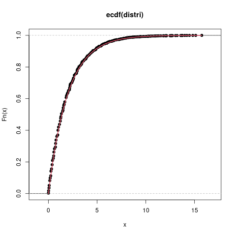
plot(ecdf(distri))
plot(function(x) pchisq(x,k-1), 0, max(distri), col=2, lwd=2, add=TRUE)
- Distribución de \(F\)
- mínimo: \(F\) = \(0\) cuando \(R_{\cdot1}\) = \(\dots\) = \(R_{\cdot k}\) = \(n\dfrac{k+1}2\)
máximo: \(F\) = \(n(k-1)\) cuando los rangos son constantes por columnas; por ejemplo,
individuo \(X_1\) \(X_2\) \(\dots\) \(X_k\) sumas \(1\) \(1\) \(2\) \(\dots\) \(k\) \(R_{1\cdot}\) \(\vdots\) \(\vdots\) \(\vdots\) \(\vdots\) \(\vdots\) \(\vdots\) \(n\) \(1\) \(2\) \(\dots\) \(k\) \(R_{n\cdot}\) sumas \(n\) \(2n\) \(\dots\) \(kn\) \(n\dfrac{k(k+1)}2\)
Ejemplo
datos crudos
individuo \(X_1\) \(X_2\) \(X_3\) \(X_4\) 1 \(5.6\) \(8.7\) \(7.2\) \(6.6\) 2 \(3.0\) \(5.6\) \(5.4\) \(5.5\) 3 \(6.6\) \(3.9\) \(9.2\) \(6.7\) 4 \(3.5\) \(5.8\) \(9.6\) \(7.8\) 5 \(3.3\) \(7.8\) \(4.0\) \(3.5\) rangos
individuo \(X_1\) \(X_2\) \(X_3\) \(X_4\) 1 1 4 3 2 2 1 4 2 3 3 2 1 4 3 4 1 2 4 3 5 1 4 3 2 \(R_{\cdot j}\) 6 15 16 13 - \(F\) = \(\dfrac {12} {5\cdot4\cdot(4+1)} \sum_{j=1}^4(R_{\cdot j}-12.5)^2\) = \(7.32\)
X = cbind (X1 = c(5.6,3.0,6.6,3.5,3.3), X2 = c(8.7,5.6,3.9,5.8,7.8),
           X3 = c(7.2,5.4,9.2,9.6,4.0), X4 = c(6.6,5.5,6.7,7.8,3.5))
(Rij = t (apply (X, 1, rank)))
(R.j = colSums (Rij))
n = nrow (X); k = ncol (X)
(F = 12/n/k/(k+1) * sum ((R.j - n*(k+1)/2) ^ 2))
1 - pchisq (F, k-1)
friedman.test (X)
X1 X2 X3 X4 [1,] 1 4 3 2 [2,] 1 4 2 3 [3,] 2 1 4 3 [4,] 1 2 4 3 [5,] 1 4 3 2 X1 X2 X3 X4 6 15 16 13 [1] 7.32 [1] 0.06236834 Friedman rank sum test data: X Friedman chi-squared = 7.32, df = 3, p-value = 0.06237- versión para casos con empates (es la implementada en R):
- \(F\) = \(\displaystyle \frac{12}{nk(k+1)-\dfrac{\sum_{i=1}^n\sum_{j=1}^{g_i}(t_{ij}^3-t_{ij})}{k-1}} \sum_{j=1}^k\left(R_{\cdot j}-\frac{n(k+1)}2\right)^2\)
- en realidad, la prueba de Friedman tiene como hipótesis nula \(H_0:(X_1,\dots,X_k)\) intercambiable \(\equiv\)
\(H_0:F_{X_1,\dots,X_k}=F_{X_{\sigma(1)},\dots,X_{\sigma(k)}}\) \(\forall\,\sigma\in S_k\), donde \(S_k\) es
el grupo de permutaciones de orden \(k\)
si la distribución conjunta no es intercambiable, no funciona bien:
## distro conjunta:
##    ##
##    ##
##  ##
##  ##
##      ##
##      ##
n <- 30
dist <- replicate(1e4,
{
    x <- runif(n,0,3)
    y <- runif(n,0,1) - (x<1) + 2*(x<2)
    friedman.test(cbind(x,y))$p.value
})
summary(dist)
mean(dist<0.05)
## > summary(dist)
##      Min.   1st Qu.    Median      Mean   3rd Qu.      Max.
## 0.0000021 0.0105871 0.0678892 0.1708853 0.2733217 1.0000000
## > mean(dist<0.05)
## [1] 0.4301
la distribución de los p-valores no es uniforme \(U(0,1)\) bajo \(H_0:F_1=\dots=F_k\)
1.5.2. Coeficiente de concordancia de Kendall
- Concordancia entre \(n\) jueces al ordenar \(k\) elementos
- \(W\) = \(\dfrac{F}{n(k-1)}\) \(\in\) \([0;1]\)
- \(W=1\) \(\iff\) concordancia total)
- \(H_0\): no existe concordancia \(\iff\) \(H_0\): \(W\approx0\)
- \(H_1\): sí existe concordancia
- RC = \([F > c]\) = \([W > h]\)
1.5.3. Respuesta binaria - Q de Cochran
- Equivale a aplicar la \(F\) de Friedman a la tabla binaria (muchos empates): Friedman's (1937) statistic, corrected for ties (…) reduces to Cochran's statistic for only two categories (see Lehmann, p. 267).
- \(\vec X\) = \((X_1,\dots,X_k)\) vector aleatorio con \(X_i\) \(\hookrightarrow\) \(\mathcal B(p_i)\)
- \(H_0\) : \(\forall\,i,j\), \(p_i=p_j\) ; \(H_1\) : \(\exists\,i,j\), \(p_i\ne p_j\)
| individuo | \(X_1\) | \(\dots\) | \(X_k\) | sumas |
|---|---|---|---|---|
| \(1\) | \(x_{11}\) | \(\dots\) | \(x_{1k}\) | \(R_{1}\) |
| \(\vdots\) | \(\vdots\) | \(\vdots\) | \(\vdots\) | \(\vdots\) |
| \(n\) | \(x_{n1}\) | \(\dots\) | \(x_{nk}\) | \(R_{n}\) |
| sumas | \(C_{1}\) | \(\dots\) | \(C_{k}\) | \(T\) |
- \(\hat p_j\) = \(\dfrac{C_j}n\)
- Se mide la dispersión de las \(\hat p_j\) o de las \(C_j\) \[S = \sum_{j=1}^k\left(C_j-\frac Tk\right)^2\] RC = \([S > c]\)
- \(\dfrac{\hat p_j-p}{\sqrt{\dfrac{p(1-p)}n}}\) \(\xrightarrow[\mathcal L]{H_0}\) \(\mathcal N(0;1)\) \(\implies\) \(\dfrac{C_j-\dfrac Tk}{\sqrt{\text{Var}(C_j)}}\) \(\xrightarrow[\mathcal L]{H_0}\) \(\mathcal N(0;1)\)
- \({\text{Var}}(C_j)\) = \(\displaystyle\sum_{i=1}^n{\text{Var}}(X_{ij})\) = \(\displaystyle\sum_{i=1}^n\dfrac{R_i}k \left(1-\dfrac{R_i}k\right)\)
- \(\widehat{\text{Var}}(C_j)\) = \(\displaystyle\sum_{i=1}^n\widehat{\text{Var}}(X_{ij})\) = \(\displaystyle\sum_{i=1}^n\dfrac{R_i}k \left(1-\dfrac{R_i}k\right)\dfrac k{k-1}\) \(\implies\) \(\displaystyle \dfrac{\left(C_j-\dfrac Tk\right)^2} {\sum_i R_i(k-R_i)\dfrac1{k(k-1)}}\) \(\xrightarrow[\mathcal L]{H_0}\) \(\chi^2_1\) \(\implies\) \(Q\) = \(k(k-1)\dfrac S{\sum_i R_i(k-R_i)}\) = \((k-1)\dfrac{\sum_{j=1}^k\left(C_j-\dfrac Tk\right)^2} {T-\sum_{i=1}^n\dfrac{R_i^2}k}\) \(\xrightarrow[\mathcal L]{H_0}\) \(\chi^2_{k-1}\) (las \(C_j\) son dependientes, \(\sum_j C_j\) = \(T\))
- RC = \([Q > c]\)
- Distribución de \(Q\)
- aproximadamente \(\chi^2_{k-1}\) si \(n > 6\) y \(nk > 24\)
- Montecarlo
- mantener \(R_i\) constantes permutando dentro del individuo
Ejemplo
individuo \(X_1\) \(X_2\) \(X_3\) \(X_4\) \(R_i\) 1 1 0 0 0 1 2 0 0 1 1 2 3 1 0 1 0 2 4 0 0 0 0 0 5 1 1 0 1 3 \(C_{j}\) 3 1 2 2 \(T=8\) X <- matrix (c(1,0,1,0,1, 0,0,0,0,1, 0,1,1,0,0, 0,1,0,0,1), 5) k <- ncol (X) R <- apply (X, 1, sum) # rowSums (X) C <- apply (X, 2, sum) # colSums (X) T <- sum (X) # == sum (C) == sum (R) (Q <- (k-1) * sum ((C - T/k) ^ 2) / (T - sum (R^2 / k))) 1 - pchisq (Q, k-1) # p-valor asintótico DescTools::CochranQTest (X) friedman.test (X) # es lo mismo Q <- function (X) { k <- ncol (X) R <- apply (X, 1, sum) # rowSums (X) C <- apply (X, 2, sum) # colSums (X) T <- sum (X) # == sum (C) == sum (R) (k-1) * sum ((C - T/k) ^ 2) / (T - sum (R^2 / k)) } ## P-valor Montecarlo mean (replicate (1e4, Q (t (apply (X, 1, sample)))) >= Q(X))
[1] 1.714286
[1] 0.6337624
2. Contrastes de independencia
2.1. Prueba \(\chi^2\)
- \(H_0:X\text{ y }Y\text{ son independientes}\), \(H_1:X\text{ y }Y\text{ son dependientes}\)
- Única prueba para independencia en general (no sólo independencia lineal).
- Para variables discretas finitas (o agrupadas).
- \(H_0:\) \(\forall\,i,j\), \(p_{ij}\) = \(\Pr[X=x_i,Y=y_j]\) = \(\Pr[X=x_i]\Pr[Y=y_j]\) = \(p_{i\cdot}p_{\cdot j}\)
- \(H_1:\) \(\exists\,i,j\), \(p_{ij}\ne p_{i\cdot}p_{\cdot j}\)
Tabla de contingencia
\(X\) \ \(Y\) \(y_1\) \(\dots\) \(y_r\) totales \(x_1\) \(n_{11}\) \(\dots\) \(n_{1r}\) \(n_{1\cdot}\) \(\vdots\) \(\vdots\) \(\vdots\) \(\vdots\) \(\vdots\) \(x_k\) \(n_{k1}\) \(\dots\) \(n_{kr}\) \(n_{k\cdot}\) totales \(n_{\cdot1}\) \(\dots\) \(n_{\cdot r}\) \(n\) - Frecuencias esperadas bajo \(H_0\): \(E_{ij}\) = \(n\dfrac{n_{i\cdot}}n\dfrac{n_{\cdot j}}n\)
- Verosimilitud bajo \(H_1\): \(\mathcal L(\vec n,\vec p_{(X,Y)})\) \(\propto\) \(\displaystyle\prod_{i=1}^k\prod_{j=1}^r p_{ij}^{n_{ij}}\) \(\implies\) EMV \(\hat p_{ij}\) = \(\dfrac{n_{ij}}n\)
- Verosimilitud bajo \(H_0\): \(\mathcal L(\vec n, \vec p_X, \vec p_Y)\) \(\propto\) \(\displaystyle\prod_{i=1}^k\prod_{j=1}^r (p_{i\cdot}p_{\cdot j})^{n_{ij}}\) = \(\displaystyle\prod_{i=1}^kp_{i\cdot}^{n_{i\cdot}}\prod_{j=1}^r p_{\cdot j}^{n_{\cdot j}}\) \(\implies\) EMV \(\hat p_{i\cdot}\) = \(\dfrac{n_{i\cdot}}n\), \(\hat p_{\cdot j}\) = \(\dfrac{n_{\cdot j}}n\)
- Razón de verosimilitudes \(\Lambda(\vec n)\) = \(\dfrac{\mathcal L(\vec n,\hat p_X,\hat p_Y)}{\mathcal L(\vec n,\hat p_{(X,Y)})}\) = \(\displaystyle\prod_{i=1}^k\prod_{j=1}^r \left(\dfrac{\dfrac{n_{i\cdot}}n\dfrac{n_{\cdot j}}n}{n_{ij}/n}\right)^{n_{ij}}\) = \(\displaystyle\prod_{i=1}^k\prod_{j=1}^r \left(\dfrac{\dfrac{n_{i\cdot}n_{\cdot j}}n}{n_{ij}}\right)^{n_{ij}}\) \(\displaystyle\prod_{i=1}^k\prod_{j=1}^r\left(\dfrac{E_{ij}}{O_{ij}}\right)^{O_{ij}}\)
- \(G\) = \(-2\ln\Lambda\) \(\xrightarrow[\mathcal L]{H_0}\) \(\chi^2_{(kr-1) - [(k-1)+(r-1)]}\) = \(\chi^2_{(k-1)(r-1)}\)
- \(D\) = \(\displaystyle\sum_{i=1}^k\sum_{j=1}^r\dfrac{(O_{ij}-E_{ij})^2}{E_{ij}}\) \(\xrightarrow[\mathcal L]{H_0}\) \(\chi^2_{(k-1)(r-1)}\)
dat <- carData::Chile[c("education","vote")]
dat$education <- factor (dat$education, levels = c ("P", "S", "PS"))
(T <- chisq.test (table (dat)))
(D <- T$statistic)
T$p.value
(O <- T$observed)
(E <- T$expected)
(R <- T$residuals)
R^2                     # residuos cuadrados
(O-E)^2 / E             # sumandos del estadígrafo
prop.table (O, 1)       # frecuencias condicionadas
	Pearson's Chi-squared test

data:  table(dat)
X-squared = 135.85, df = 6, p-value < 2.2e-16
X-squared
 135.8485
[1] 7.528046e-27
         vote
education   A   N   U   Y
       P   52 266 296 422
       S  103 397 237 311
       PS  32 224  52 130
         vote
education        A        N        U        Y
       P  76.81681 364.3664 240.3093 354.5075
       S  77.70658 368.5868 243.0928 358.6138
       PS 32.47661 154.0468 101.5979 149.8787
         vote
education           A           N           U           Y
       P  -2.83150838 -5.15320625  3.59250661  3.58461538
       S   2.86931756  1.47995902 -0.39077765 -2.51431295
       PS -0.08363231  5.63613432 -4.92063527 -1.62374326
         vote
education            A            N            U            Y
       P   8.017439725 26.555534611 12.906103747 12.849467427
       S   8.232983270  2.190278705  0.152707169  6.321769613
       PS  0.006994362 31.766010103 24.212651488  2.636542188
         vote
education            A            N            U            Y
       P   8.017439725 26.555534611 12.906103747 12.849467427
       S   8.232983270  2.190278705  0.152707169  6.321769613
       PS  0.006994362 31.766010103 24.212651488  2.636542188
         vote
education          A          N          U          Y
       P  0.05019305 0.25675676 0.28571429 0.40733591
       S  0.09828244 0.37881679 0.22614504 0.29675573
       PS 0.07305936 0.51141553 0.11872146 0.29680365
- Cuando \(k=r=2\) es habitual (el
chisq.testdeRlo hace por omisión) aplicar la corrección por continuidad o de Yates para mejorar la aproximación asintótica: \(D\) = \(\displaystyle\sum_{i=1}^k\sum_{j=1}^r\dfrac{(|O_{ij}-E_{ij}|-\frac12)^2}{E_{ij}}\)
2.2. Pruebas de correlación
- Para variables al menos ordinales.
- \(\overrightarrow{(X,Y)}\) = \(\bigl((X_1,Y_1),\dots,(X_n,Y_n)\bigr)\) muestra de \((X,Y)\)
- \(H_0\) : \(X\) y \(Y\) son (linealmente) independientes
2.2.1. Correlación de Pearson
- \((X,Y)\) \(\hookrightarrow\) \(\mathcal N_2(\vec\mu;\Sigma)\) \(\implies\) independencia \(\equiv\) correlación lineal nula\
- \(H_0\) : \(X\) y \(Y\) independientes \(\iff\) \(\rho_{XY}=0\)
- EMV de \(\rho\): \(R\) = \(\dfrac{S_{XY}}{S_{X}S_Y}\)
- RC = \([R^2 > c]\) = \(\left[\dfrac{(n-2)R^2}{1-R^2} > h\right]\)
- \((X,Y)\) \(\hookrightarrow\) \(\mathcal N_2(\vec\mu;\Sigma)\) \(\implies\) \(\dfrac{(n-2)R^2}{1-R^2} \) \(\stackrel{H_0}{\hookrightarrow}\) \(F_{1,n-2}\) \(\iff\) \(\sqrt{\dfrac{(n-2)R^2}{1-R^2}}\) \(\stackrel{H_0}{\hookrightarrow}\) \(t_{n-2}\)
plot (mtcars$qsec, mtcars$mpg)
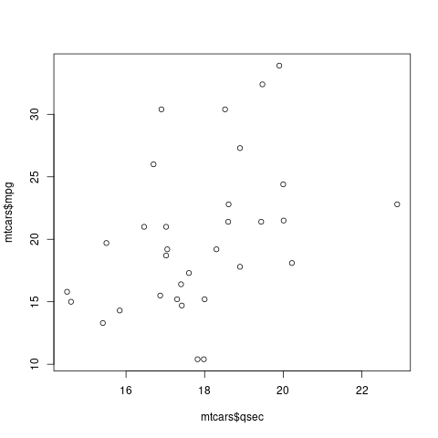
cor.test (mtcars$qsec, mtcars$mpg)
	Pearson's product-moment correlation

data:  mtcars$qsec and mtcars$mpg
t = 2.5252, df = 30, p-value = 0.01708
alternative hypothesis: true correlation is not equal to 0
95 percent confidence interval:
 0.08195487 0.66961864
sample estimates:
     cor
0.418684
2.2.2. Correlación de Spearman
- Para variables
- cualitativas ordinales
- rangos de cuantitativas \(\implies\) robustez
- Es el coeficiente de Pearson aplicado a rangos: \(R_s\) = \(\dfrac{\text{Cov}(R_X,R_Y)}{\sqrt{\text{Var}(R_X)\text{Var}(R_Y)}}\) = \(1-\dfrac{6\sum_{i=1}^n(R_{X,i}-R_{Y,i})^2}{n(n^2-1)}\)
- RC = \([|R_s| > c]\)
- \(\sqrt{n-1}R_s\) \(\xrightarrow[\mathcal L]{H_0}\) \(\mathcal N(0;1)\)
plot (rank(mtcars$qsec), rank(mtcars$mpg))
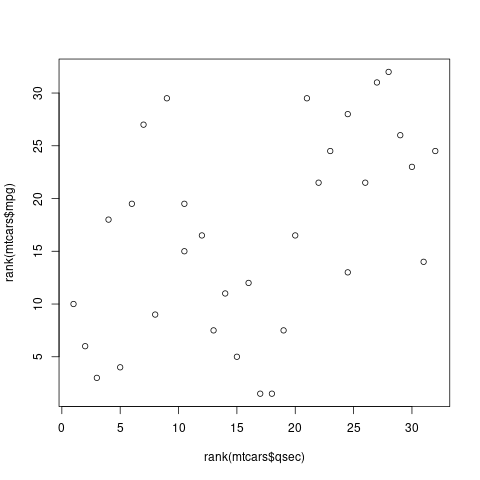
cor.test (mtcars$qsec, mtcars$mpg, method="spearman")
	Spearman's rank correlation rho

data:  mtcars$qsec and mtcars$mpg
S = 2908.4, p-value = 0.007056
alternative hypothesis: true rho is not equal to 0
sample estimates:
      rho
0.4669358
3. Prueba exacta de Fisher
- Alternativa exacta a la prueba \(\chi^2\) de homogeneidad o independencia.
- Usa la distribución exacta multihipergeométrica de la \(D\) de Pearson.
- Habitual para tablas \(2\times2\) salvo si las frecuencias observadas son grandes.
- En tablas mayores suele usarse una aproximación de Montecarlo.
fisher.test (table (mtcars [c("am","cyl")])) # exacto
(T <- table(dat)) # Chile
fisher.test (T) # error
fisher.test (T, simulate.p.value=TRUE) # Montecarlo
fisher.test (T, simulate.p.value=TRUE, B=1e4)
	Fisher's Exact Test for Count Data

data:  table(mtcars[c("am", "cyl")])
p-value = 0.009105
alternative hypothesis: two.sided
         vote
education   A   N   U   Y
       P   52 266 296 422
       S  103 397 237 311
       PS  32 224  52 130
Error in fisher.test(T) :
  FEXACT error 6.  LDKEY=606 is too small for this problem,
  (ii := key2[itp=402] = 467019147, ldstp=18180)
Try increasing the size of the workspace and possibly 'mult'

	Fisher's Exact Test for Count Data with simulated p-value (based on 2000 replicates)

data:  T
p-value = 0.0004998
alternative hypothesis: two.sided

	Fisher's Exact Test for Count Data with simulated p-value (based on 10000 replicates)

data:  T
p-value = 9.999e-05
alternative hypothesis: two.sided
4. Riesgo relativo (RR) y razón de cuotas (odds ratio OR)
- situación del contraste de homogeneidad (dos poblaciones independientes)
- cuantificar efecto de factor sobre probabilidad de enfermar
- factor: \(F\) = fuma ; \(N\) = no
- \(E\) = enfermo ; \(S\) = sano
| \(E\) | \(S\) | ||
|---|---|---|---|
| \(F\) | \(a\) | \(b\) | \(n_F\) |
| \(N\) | \(c\) | \(d\) | \(n_N\) |
| \(n_E\) | \(n_S\) | \(n\) |
- riesgo de fumar \(p_F\) = \(\Pr[E\mid F]\), \(\hat p_F\) = \(\dfrac a{n_F}\)
- riesgo de no fumar \(p_N\) = \(\Pr[E\mid N]\), \(\hat p_N\) = \(\dfrac b{n_F}\)
4.1. riesgo relativo
- riesgo relativo RR = \(\dfrac{p_F}{p_N}\)
- si el factor no influye, entonces RR = \(1\)
- si el factor es de riesgo, RR \( > \) \(1\)
- si el factor es de prevención, RR \( < \) \(1\)
- estimador \(\widehat{\text{RR}}\) = \(\dfrac{\hat p_F}{\hat p_N}\) = \(\dfrac{a/n_F}{c_/n_N}\)
- ventaja del RR: interpretación fácil
inconveniente:
no calculable en muestreos diseñados (caso-control) pues
- se conoce \(\Pr[F\mid E]\)
- se desconoce \(\Pr[E]\)
- no se puede calcular \(\Pr[E\mid F]\)
4.2. razón de cuotas (odds ratio)
- cuota (odds) de un suceso de probabilidad \(p\) es \(\dfrac p{1-p}\)
- razón de cuotas = odds ratio = OR = \(\dfrac{\dfrac{p_F}{1-p_F}}{\dfrac{p_N}{1-p_N}}\) \(\implies\) \(\widehat{\text{OR}}\) = \(\dfrac{\dfrac{a/(a+b)}{b/(a+b)}}{\dfrac{c/(c+d)}{d/(c+d)}}\) = \(\dfrac{ad}{bc}\)
- \(p_F\), \(p_N\) \(\approx\) \(0\) \(\implies\) OR \(\approx\) RR
- no cambia si se considera la matriz traspuesta: \(\dfrac{\dfrac{\widehat\Pr[F\mid E]}{\widehat\Pr[N\mid E]}} {\dfrac{\widehat\Pr[F\mid S]}{\widehat\Pr[N\mid S]}}\) = \(\dfrac{\dfrac{a/(a+c)}{c/(a+c)}}{\dfrac{b/(b+d)}{d/(b+d)}}\) = \(\dfrac{ad}{bc}\) = \(\widehat{\text{OR}}\)
4.3. ejemplo
datos: E = enfermedad coronaria ; F = fuma
E S F 84 2916 N 87 4913
X <- matrix (c(4913,2916,87,84), 2,
             dimnames=list(factor=c("N","F"),salud=c("S","E")))
epitools::riskratio (X) # ojo al orden; existe opción "rev"
epitools::riskratio (t (X)) # incorrecto
epitools::oddsratio (X)
epitools::oddsratio (t (X))